In the age of big data we often find ourselves facing CPU-intensive data processing tasks, therefore it is useful to understand how to harness all available CPU power to tackle a particular problem.

Recently we came across a Python script which was CPU-intensive, but when the analyst viewed their overall CPU usage it was only showing ~25% utilization. This was because the script was only running in a single process, and therefore only fully utilizing a single core. For those of us with a few notches on our belts, this should seem fairly obvious, but I think it is a good exercise and teaching example to talk about the different methods of multi-core/multi-node programming in Python.

This isn’t meant to be an all-encompassing tutorial on multi-core and distributed programming, but it should provide an overview of the available approaches in Python.

Download the Python scripts »

The Problem:

Throughout this tutorial, we’ll use a simple problem as an example:

The problem is to generate N random integers, and calculate the sum of the generated integers.

This is a completely contrived example, but it will act as a simple job that can easily be distributed. It should be clear to the reader that the computational complexity of this problem is O(N), and that the time required to solve the problem will scale linearly as N grows.

sumValues.py

— GIST https://gist.github.com/myover/0295871401ff3ebbb2daa1f4b67e249e.js —

The Multi-Core Approach:

As the old adage goes, “Many cores make light work”, or something like that right? More than likely, any modern desktop or even laptop today is going to have at least 2-4 cores available, so let’s take advantage of that and cut down our total compute time for CPU intensive tasks. First, I should mention that not every program can achieve equivalent speed increase by distributing the load. While the details of calculating the speedup parallel computation will provide is beyond the scope of this post, it’s enough to understand some programs or functions are more “parallelizable” than others. In general, computations with a high degree of independence will benefit most from these parallel computing methods.

Pro Tip: Some programs or functions are more “parallelizable” than others. In general, computations with a high degree of independence will benefit most from these parallel computing methods.

The Multi-Core Approach:

The multiprocessing package has been available as of Python 2.6, and provides a relatively simple mechanism for creating a sub-process. IMHO, this is much simpler than using threading, which we’ll leave as an exercise for the reader to explore.

So let’s show how we could approach this problem with multiprocessing.

processApproach.py

— GIST https://gist.github.com/myover/ccfaeb032b3bca3a0b7556de4da5fcf1.js —

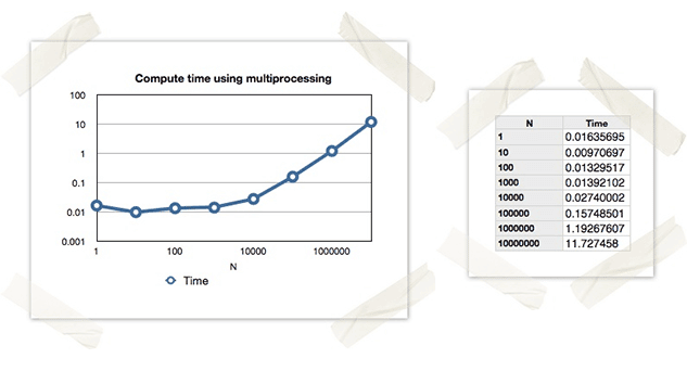
A few things should stand out from these results:

1. At higher values of N, we received an approximate 2x decrease in computation time. This is what we expected, as we were spreading the work over 2 cores.
2. At lower values of N, we see that we’re not achieving a proportional decrease in work, and in most cases we’re actually performing worse than before. This is due to the additional overhead we’re adding by creating new processes, which shows that parallel programming is not always appropriate.

Caveat Emptor: Parallel programming is not always appropriate. For low volumes of work it can actually lead to a performance decrease.

Take a little time to read through the code in this example and compare it to the the original direct approach. You’ll notice that we’ve added a new function doWork which takes two arguments: N and q. N is the number of values to sum together, and q is a Queue object which we’ll use to pass the result back to the calling process. Next you’ll notice in __main__ we’ve created four separate processes (p1-p4), each receiving an equal portion of the work (N/4). Each of these gets kicked off by calling .start() then we collect the results from the queue using q.get(True). Note that in this case we know that we’re waiting for exactly four values from the queue, so we use blocking=True to wait until we receive exactly four values. Take some time to reference the Python Docs on multiprocessing to sort out any issues you still have questions on before we move on.

Take a dip in the Pool

In the previous example we saw the advantages of using multiple processes using multiprocessing and Process. You may have already noticed, but explicitly creating multiple processes is a bit cumbersome. In the next example we demonstrate Pool, another class in the multiprocessing package. With pool you can alleviate much of the coding overhead of creating multiple processes for the same function. As shown in the example below, you can simply define the number of worker processes you want to create in the pool, then pass an iterable object containing the parameters for each process. Note that in this example we’ve paired things up exactly, 4 workers with 4 mapped processes, but in practice you could have any number of mapped processes, you’re not constrained by the number or worker processes in any way.

poolApproach.py

— GIST https://gist.github.com/myover/5bffac54cfe0e2c8b04fb9cdfa7bcd0c.js —

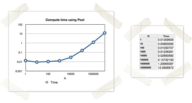
Note that these results look approximately equivalent to the previous Process example, but the code is much cleaner IMHO.

You should notice that this is about the same as the previous example using multiple Process instances, but the code is a bit cleaner and easier to read. In this example, we’ve gotten rid of the Queue object, and pass the result back using the return value. In __main__ you’ll see that we create a pool instance using Pool(processes=4). This creates a pool of 4 worker nodes, which we can then send work to in several ways. Next we call pool.map(doWork, (N/4,N/4,N/4,N/4)), which creates 4 jobs to be processed on the 4 worker processes available in the pool. We’ve chosen to use pool.map, but we leave it as an exercise for the reader to look at the other synchronous and asynchronous methods for sending work to the worker processes. The first argument to Pool.map is the function we want to execute within the new process, and the second argument is an iterable object which contains arguments for each new process we spawn. Here we’re calling doWork, which takes a single argument (N), and passing a Tuple with 4 elements. Since we are passing 4 arguments in the tuple, this will create 4 separate calls to doWork, each with the argument N/4. It should be clear, but since we’re creating 4 processes, we’re splitting the work up evenly, with each adding N/4 integers. This is the same amount of total work as the first example, which sums N integers.

Taking it to the cloud

The previous examples have shown a few simple methods of spreading work across multiple cores of a single system. This is effective for large jobs, but when dealing with very large data sets it may be necessary to take it the next level and try multi-node processing or “cloud computing”. This will allow you to distribute work across multiple networked nodes, and utilize their CPUs as well as their additional memory and disk resources. The details of these frameworks are beyond the scope of this post, but we’ve found Celery very useful for this kind of distributed processing. Celery requires a small amount of setup, but isn’t much more difficult to use than either of the examples shown in this post. Once Celery is setup and configured, you simply need to add a decorator to the top of functions that you want to run on distributed nodes which will cause them to be added to the task queue and farmed out to worker nodes when they’re called. If you’re interested in learning more about Celery, you can find some useful tutorials here.

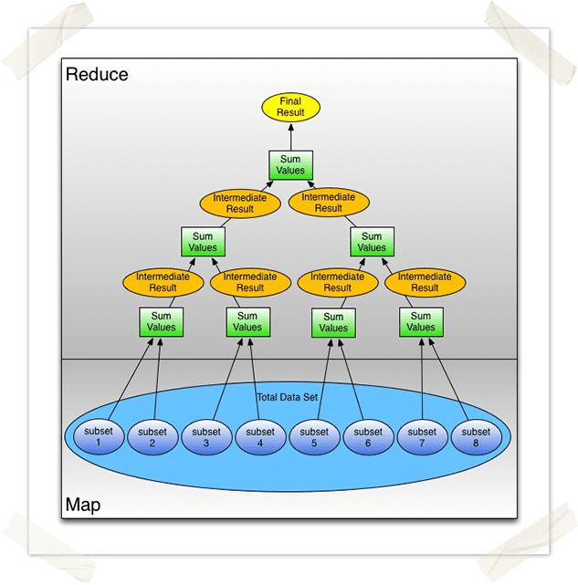
You may have also heard the concept of Map-Reduce, which is quite similar to the example shown here. Map-Reduce is used for a specific type of parallel programming known as embarrassingly parallel workloads. These types of workloads can be split into separate parallel tasks with little or no effort. Map-Reduce has two steps: Map, which splits the task into parallel tasks, and Reduce, which reduces the input data set into a reduced (or single) set of outputs. In many cases the reduce function is designed to be associative, which allows for massively parallel processing. This is achieved by computing results in “tiers”, where intermediate results are computed, then the intermediate calculations are reduced further by performing the reduce step on their results. If you’d like to try out Map-Reduce for large data sets, here are few frameworks to check out (in no particular order): Hadoop, CouchDB, MongoDB, Cassandra, Amazon EMR

Pro Tip: For very large data sets, consider using multi-node parallel processing frameworks such as the Celery task queue or a Map-Reduce framework.

Warning: While it’s good for practice, using these distributed processing frameworks for small data sets is probably overkill. Remember that not every problem can be solved more efficient in parallel, and sometimes the additional overhead can actually decrease performance.

Conclusion

Although the task of adding random numbers is a bit contrived, these examples should have demonstrated the power of and ease of multi-core and distributed processing in Python. Parallel processing does not always provide increased performance, however many tasks can benefit from careful task splitting. Furthermore, most consumer computers today have multiple cores available, so writing a single-process program is the wrong way to approach CPU intensive workloads. Once you’re comfortable writing multi-process programs, step it up and try your hand at multi-node processing using Celery for Python or one of the many Map-Reduce frameworks.

Additional References

• http://docs.python.org/library/multiprocessing.html
• http://stackoverflow.com/questions/203912/does-python-support-multiprocessor-multicore-programming