

We see huge benefits of machine learning in the field of computer security.
Much of the work we do on a daily basis can be automated and classified by a machine, leaving us to focus on more interesting and challenging problems. One stunning example is the automated binary exploitation and patching research funded by DARPA for the Cyber Grand Challenge. Problems like these are the stepping stones that will lead us to a future of automated computer security.
To encourage future candidates (and ourselves) to delve into the world of machine learning, we built a new technical challenge to test the waters. The challenge is based on a CTF problem from SECCON, discovered by @ctfhacker, and features a mysterious compiler that always produces unique binaries.
In this post, I’ll be describing my sample solution to the “Machine Learning Binaries” challenge. The crux of the challenge is to build a classifier that can automatically identify and categorize the target architecture of a random binary blob. If you’d like to play the challenge yourself, head over to our Machine Learning Binaries tech challenge and start capturing samples.
Example code for connecting to the server on GitHub:
— GIST https://gist.github.com/gitpraetorianlabs/989736b1e655b986bac9.js —
I’ve written a sample solution, which uses high-level machine learning primitives from the scikit learn library. The write-up below is intended to spur your interest in the subject and push you in the right direction when creating a solution.
Please note: solutions to the MLB challenge must implement low-level machine learning primitives or be heavily commented if you intend on submitting to [email protected].
Ten Thousand Ft. View
Our server generates a random program and compiles it under a random instruction set architecture (ISA). The available architectures are provided by the wonderfully versatile cross compiler: crosstool-ng. Once compiled, the server selects a random section of instruction aligned code (this matters later). Given this random section of code, the challenge is to identify the original ISA from a list of possible ISAs provided by the server. We could attempt to disassemble the binary blob under each provided architecture and build heuristics to identify the likely ISA. But this is a machine learning challenge! We can just collect a bunch of data, select some key features, train a classifier, and let the machine do all our hard work.
Our MLB challenge, however strange it may seem, is actually just a text classification puzzle in disguise! We have a corpus of data that needs to be sorted into a fixed number of categories. If we treat the binary blobs as if they were just some unknown language, we can apply text-based classification principles to our problem and avoid re-inventing the wheel. Below, I’ve provided an algorithmic cheat-sheet from the documentation of scikit-learn, the framework we used in our solution.
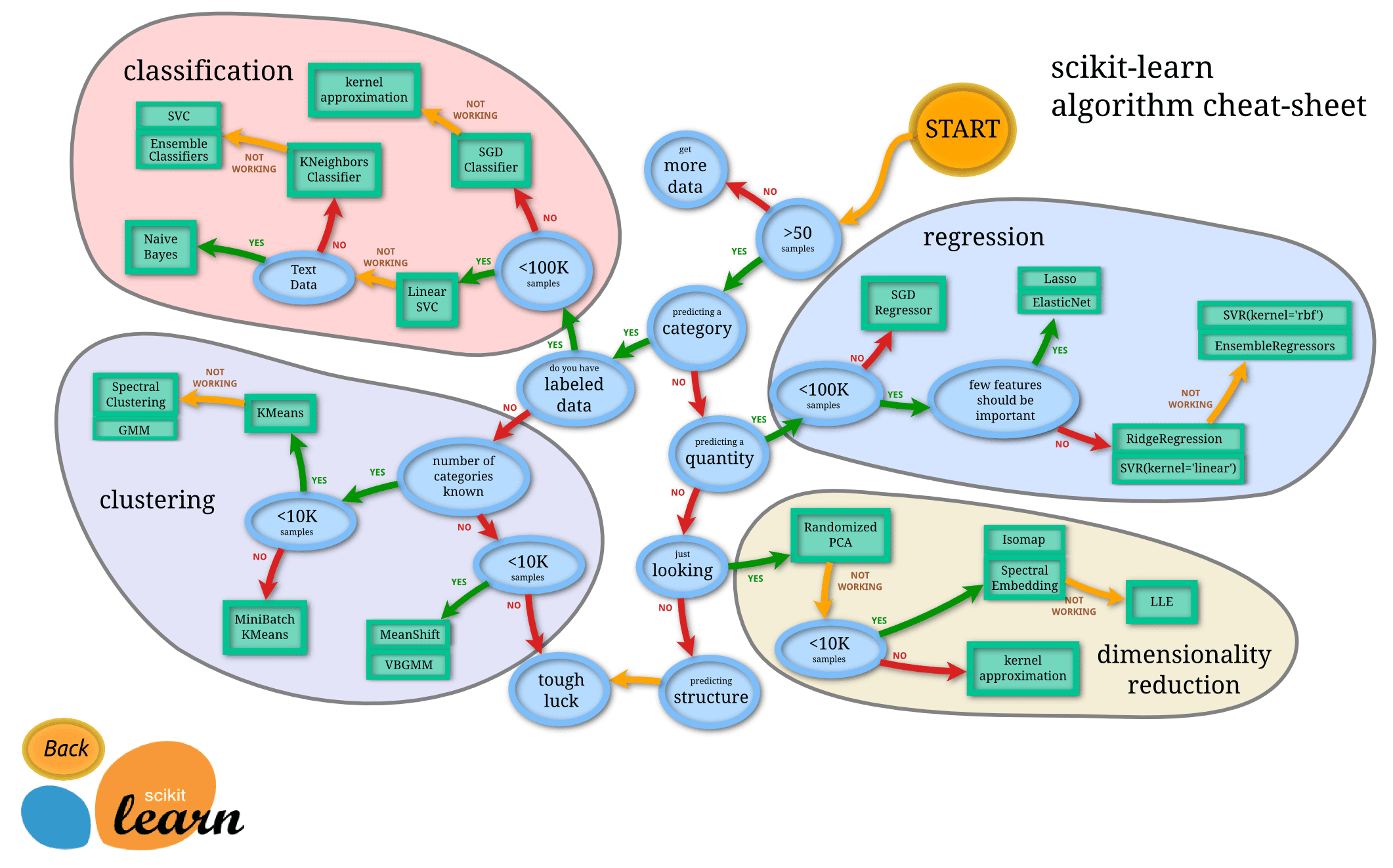
Into the Weeds
As you can see, our problem falls directly into the classification bucket, likely around the Linear SVC or Naive Bayes groups. Let’s assume we’ve collected samples of binary data. The first thing we’ll need to do though is transform the raw binary data to vectors for processing. To make things simple, we’ll convert the binary data to hex and just treat to hex characters as a “word”.
import binascii# assume we've already collected samples# this is left as an exercise to the readerdata_train = [ "x00xa0", "xb0x41", ... ] # array of binary datatarget_train = [ "avr", "x86_64", ... ] # ISA class of data# transform data to hexhex_train = [binascii.hexlify(e) for e in data_train]
Now that we’ve transformed the data, we’ll feed it through a CountVectorizer from the scikit library. This effectively performs frequency analysis on the input data and constructs a vector of frequencies for each input. Because each input will likely have few features, the CountVectorizer returns a sparse matrix (i.e. an optimized matrix to represent columns with many zeroes).
from sklearn.feature_extraction.text import CountVectorizervec_opts = {"ngram_range": (1, 4), # allow n-grams of 1-4 words in length (32-bits)"analyzer": "word", # analyze hex words"token_pattern": "..", # treat two characters as a word (e.g. 4b)"min_df": 0.5, # for demo purposes, be very selective about features}v = CountVectorizer(**vec_opts)X = v.fit_transform(hex_train, target_train)for feature, freq in zip(v.inverse_transform(X)[0], X.A[0]):print("'%s' : %s" % (feature, freq))
We specified a very selective min_df, which drops features that do not meet a specific frequency requirement. In the real solution, the min_df should be tuned for accuracy, but we just want to see a sample of the data. The three features in this sample data are shown below:
'00' : 90'20' : 35'00 00' : 2
Next, it’s helpful to normalize our data with respect to the corpus of documents. A popular technique to normalize document vectors is Tf–idf, or “term frequency–inverse document frequency”. Our CountVectorizer has given us the term frequency of tokens within our corpus, however, this over emphasizes common terms among all documents. For example, almost every ISA will likely contain null bytes throughout the binary, just as you could find the word “the” within most English documents. Inverse document frequency will allow us to de-emphasize these terms common to all documents and focus on the terms with more meaning (e.g. x20 in our sample). Again, we’ll turn to scikit for an implementation of tf-idf.
from sklearn.feature_extraction.text import TfidfTransformeridf_opts = {"use_idf": True}idf = TfidfTransformer(**idf_opts)# perform the idf transformX = idf.fit_transform(X)
At this point, you may have noticed a pattern in our process. We massage the data by applying transforms, one after another. Since this is a common pattern of text analysis, scikit has support for a streamlined method of chaining transforms together called a pipeline.
from sklearn.pipeline import Pipelinepipeline = Pipeline([('vec', CountVectorizer(**vec_opts)),('idf', TfidfTransformer(**idf_opts)),])X = pipeline.fit_transform(hex_train, target_train)
The output of our pipeline is now a normalized term frequency vector for each document. As a demonstration, we can use Principal Component Analysis (PCA) to create a scatter plot of our vectors in a two dimensional space. To my understanding, PCA isn’t the best tool for the large sparse matrices we’re dealing with, but it does paint a picture of our data.
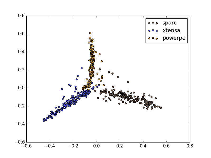
As you can see, there are very strong distinctions between the three ISAs in the image above. From this point, we simply have to choose a classifier and begin training! I’ll leave classifier selection and hyper-parameter tweaking as an exercise to the reader. Hopefully this is enough to get you interested in our technical challenge.
Best of luck!